I used to play the clarinet and I'm a big fan of music but this article is not about that. I also used to listen to static noise by adjusting radio frequencies but this is not about that either.
Ronald H. Coase, a renowned British Economist once said "If you torture the data long enough, it will confess to anything". In this piece, I will walk us through a step by step guide to torturing data efficiently. Let's go!

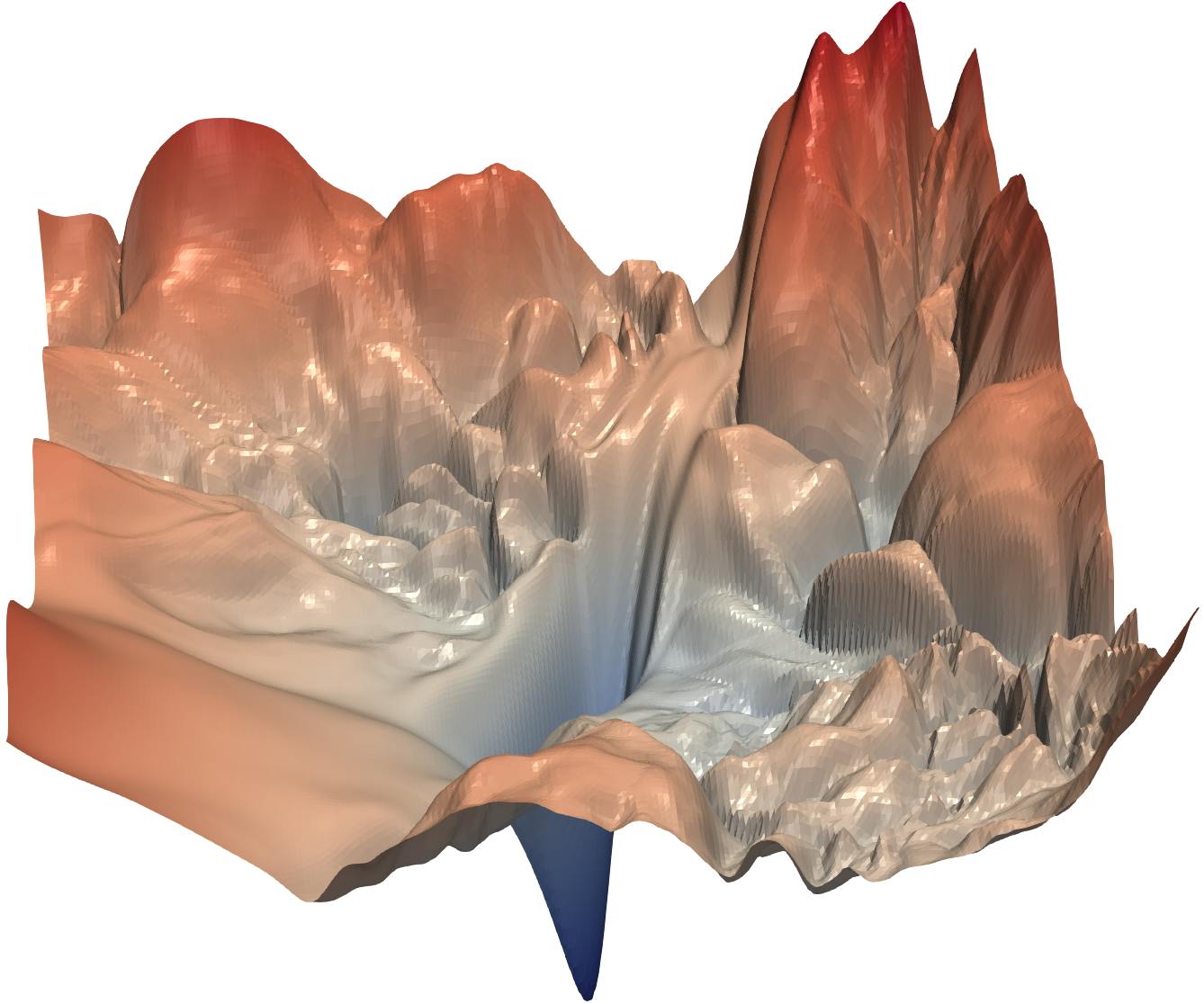
Manual tuning is a huge pain for the ML Engineer. The image above (for those who do not know) is a depiction of the loss landscape. Depending on your initial parameters, you could end up starting at any point in that landscape. Your goal is to have made your way to the global minimum of your search space at the end of the tuning process. Though the human brain is undisputedly powerful, this is nigh impossible via manual tuning.
I mean, you'll first have to think up a strategy. Do I change all parameters per training run or use the one factor at a time approach? The sad truth is that this is a fool’s errand. The next question is, "how do I tackle this problem?"
Introducing...drum roll...
The KerasTuner
KerasTuner is an easy-to-use, scalable hyperparameter optimization framework that solves the pain points of hyperparameter search. Simply put, it helps with getting the best hyperparameters within a predefined search space for your model. The API provides access to tuners that use Bayesian Optimization, Hyperband, and Random Search algorithms. As you may have guessed, it is most useful for Tensorflow models. Let’s get technical.
Installing the KerasTuner
try:
  import kerastuner as kt
except:
  !pip install -q -U keras-tuner
  import kerastuner as kt
The code snippet above helps with the installation of the Keras Tuner. The key part—on the first run—is the except block.
There we use the good 'ol pip package with a few arguments. The -q argument just means quiet (to control the console log level) while the -U argument upgrades the package to the latest available version.
I have grown accustomed to setting up my installation with the try-except block so that I get to run the same Jupyter cell without edits regardless of whether my goal is just importing or also installing.
Importing other required libraries
In the code snippet below, we import other libraries that will be used. If you don't have any of them in your development environment, run pip install [package name] in a terminal.
import json
import numpy as np
from sklearn.model_selection import train_test_split
import tensorflow.keras as keras
import matplotlib.pyplot as plt
from numpy.random import seed
from tensorflow import random
from keras.callbacks import EarlyStopping
from sklearn import metrics
Loading the Fashion MNIST Dataset
We will be using the fashion MNIST dataset to explore the tuner. This dataset is pretty much like the digits MNIST but instead of numbers, we have 10 fashion items. It was created because there was too much focus on the already easy MNIST digits dataset. Below is an image of samples from the dataset with every 3 rows containing a separate class.

Labels
Each training and test example is assigned to one of the following labels:
| Label | Description |
| 0 | T-shirt/top |
| 1 | Trouser |
| 2 | Pullover |
| 3 | Dress |
| 4 | Coat |
| 5 | Sandal |
| 6 | Shirt |
| 7 | Sneaker |
| 8 | Bag |
| 9 | Ankle boot |
(X_train, y_train), (X_test, y_test) = keras.datasets.fashion_mnist.load_data()
# summarize loaded dataset
print(f'Train: X = {X_train.shape}, y ={y_train.shape}')
print(f'Test:  X = {X_test.shape}, y ={y_test.shape}')
Next, we split the dataset into training and validation sets.
X_train, X_valid, y_train, y_valid = model_selection.train_test_split(
    X_train, y_train, test_size=0.2, stratify=y_train, random_state=42)
Sample Model
Below is a simple 3 layered Keras model depicting how one could normally start the parameter tuning process.
model = keras.Sequential([
    # input layer
    keras.layers.Flatten(),

    # 1st hidden layer
    keras.layers.Dense(units=512, activation="relu", kernel_regularizer=keras.regularizers.l2(0.001)),
    keras.layers.Dropout(0.5),

    # 2nd hidden layer
    keras.layers.Dense(units=256, activation="relu", kernel_regularizer=keras.regularizers.l2(0.001)),
    keras.layers.Dropout(0.5),

    # 3rd hidden layer
    keras.layers.Dense(units=128, activation="relu", kernel_regularizer=keras.regularizers.l2(0.001)),
    keras.layers.Dropout(0.5),

    # 1st output layer
    keras.layers.Dense(10, activation="softmax")
])

# compile network

model.compile(optimizer=keras.optimizers.Adam(learning_rate=0.001),
            loss=keras.losses.SparseCategoricalCrossentropy(from_logits=True),
            metrics=['accuracy'])

stop_early = keras.callbacks.EarlyStopping(monitor='val_loss', patience=5)

model.fit(X_train, y_train,
            validation_data=(X_valid, y_valid),
            epochs=10,
            callbacks=[stop_early],
            )
After running this for 10 epochs, we are only able to achieve a 71.82% accuracy. This will be compared to the results from the optimization techniques we will try out.
The Optimizers
We shall investigate the performance of all 3 built-in optimizers on a simple 3 layered multi-layer perceptron in Keras.
The first step is building the hyper model.
The Hyper Model
The hyper model is a python function that takes in the hyperparameter object hp as an argument. This then helps with defining various aspects of the search space. After this, the function returns the compiled model.
def model_builder(hp):
    # build the network architecture
    units1=hp.Int('units_1', 512, 2048, step=64)
    units2=hp.Int('units_2', 256, 1024, step=64)
    units3=hp.Int('units_3', 128, 768, step=32)

    model = keras.Sequential([
        # input layer
        keras.layers.Flatten(),

        # 1st hidden layer
        keras.layers.Dense(units=units1, activation="relu", kernel_regularizer=keras.regularizers.l2(0.001)),
        keras.layers.Dropout(0.5),

        # 2nd hidden layer
        keras.layers.Dense(units=units2, activation="relu", kernel_regularizer=keras.regularizers.l2(0.001)),
        keras.layers.Dropout(0.5),

        # 3rd hidden layer
        keras.layers.Dense(units=units3, activation="relu", kernel_regularizer=keras.regularizers.l2(0.001)),
        keras.layers.Dropout(0.5),

        # 1st output layer
        keras.layers.Dense(10, activation="softmax")
    ])

    # compile network
    hp_learning_rate = hp.Choice('learning_rate', values=[1e-2, 1e-3, 1e-4])

    model.compile(optimizer=keras.optimizers.Adam(learning_rate=hp_learning_rate),
                loss=keras.losses.SparseCategoricalCrossentropy(from_logits=True),
                metrics=['accuracy'])
    return model
After defining the function and its single argument hp, the first thing we do is define the search space for each unit. This part is arbitrary, as the limits and steps depend on personal choices. Since the units are integers, the hp.int() function is used. The start, stop and end values are set.
Next. we move on to define the model pipeline. A sequential model is used and dropouts of 0.5 are added after each layer. Of course, this can also be tuned if you wish. The same goes for the activation function and kernel regularizer used in each layer which is set to relu and l2 regularization of 0.001.
The last layer outputs the probabilities for each class and uses a softmax activation function.
Next, we define the options for the learning rate and use the hp.Choice() method. The hp.Float() method could work but it is less direct.
Finally, we compile the model with an Adam optimizer, Sparse Categorical Cross-Entropy loss and metric set as accuracy.
The Random Search
After building the model, the next step is defining the tuner. The first one we will be considering is the Random Search. As you would have guessed, this pretty much picks pseudo-random sets of hyperparameters from the search space and hopes that they give good results. It is a very useful approach if one is running a reasonable number of trials and if the model is feeling lucky.
tuner = kt.tuners.RandomSearch(model_builder,
                                objective='val_accuracy',
                                max_trials=25,
                                directory='.',
                                project_name='random_search'
                                )

stop_early = keras.callbacks.EarlyStopping(monitor='val_loss', patience=5)
Setting up the tuner is not complicated. Here, we just add in the hyper model function, include the optimization objective which is the validation accuracy and set a maximum number of trials. After these, the directory for caching results and the project name are set.
The EarlyStopping function is also defined and is set to monitor validation loss and wait for just 5 epochs.
tuner.search(X_train, y_train,
            validation_data=(X_valid, y_valid),
            epochs=10,
            callbacks=[stop_early],
            )

# Get the optimal hyperparameters
best_hps=tuner.get_best_hyperparameters(num_trials=1)[0]

print("The hyperparameter search is complete.")
print(best_hps.get_config()['values'])
Next, the tuner.search method is called. This is pretty much like the model.fit function in Keras.
the tuner.get_best_hyperparameters is called to get and display the best hyperparameters at the end of the tuner's search. The results are displayed below.
Best val_accuracy: 0.8577499985694885
Total elapsed time: 00h 24m 01s

The hyperparameter search is complete.

{'learning_rate': 0.0001, 'units_1': 1088, 'units_2': 1024, 'units_3': 640}
The Bayesian Optimizer
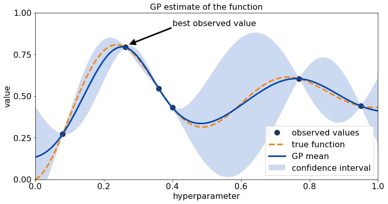
Bayesian Optimization runs models many times with different sets of hyperparameter values and evaluates past model's information to select hyperparameter values to build newer ones. This allows it to—very quickly—determine the most accurate model architecture.

tuner = kt.tuners.bayesian.BayesianOptimization(model_builder, objective='val_accuracy',max_trials=25,directory='.',project_name='bayesian_mlp')

stop_early = keras.callbacks.EarlyStopping(monitor='val_loss', patience=5)
The Tuner and EarlyStopping function are defined like before with the difference being the kt.tuners.bayesian.BayesianOptimization function selected instead as well as the project_name.
tuner.search(X_train, y_train,
            validation_data=(X_valid, y_valid),
            epochs=10,
            callbacks=[stop_early],
            )

# Get the optimal hyperparameters
best_hps=tuner.get_best_hyperparameters(num_trials=1)[0]

print("The hyperparameter search is complete.")
best_hps.get_config()['values']
This block of code where the search is implemented is pretty much the same as that of the random search. The results are shown below.
Best val_accuracy: 0.8615833520889282

The hyperparameter search is complete.

{'learning_rate': 0.0001, 'units_1': 1536, 'units_2': 1024, 'units_3': 608}
The Hyperband
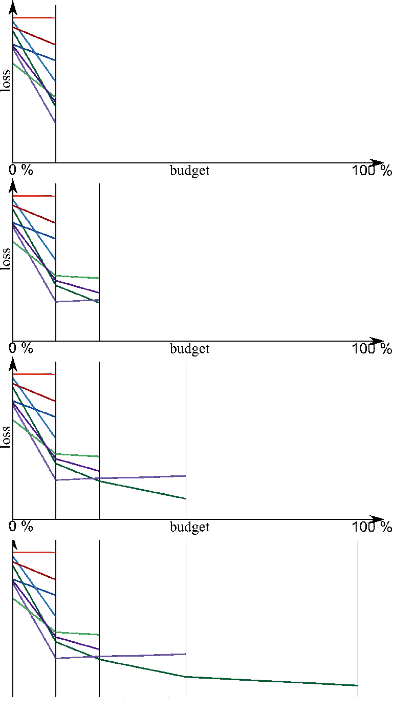
The hyperband tuning algorithm focuses on speeding up random search through adaptive resource allocation and early-stopping. Here, hyperparameter optimization is formulated as a pure-exploration non-stochastic infinite-armed bandit problem where a predefined resource like iterations, data samples, or features are allocated to randomly sampled configurations.
What does all this mean? The hyperband algorithm simply tries out several options with low resources and increases the resource allocation for those trials that seem promising. It thus successively halves the number of trials till we end up with a pretty great single solution.

tuner = kt.Hyperband(model_builder,
                     objective='val_accuracy',
                     max_epochs=10,
                     directory='.',
                     project_name='hyperband',
                     overwrite= True
                 )
stop_early = keras.callbacks.EarlyStopping(monitor='val_loss', patience=5)
We start by defining the kt.Hyperband function and a couple of its arguments. One is the previously defined hyper model model_builder. Next, the objective is set as val_accuracy which refers to the validation accuracy. This is followed by setting the maximum number of epochs max_epochs, directory and project_name. The final argument overwrite is set to True.
The EarlyStopping function is also defined as usual.
tuner.search(X_train, y_train,
            validation_data=(X_valid, y_valid),
            epochs=100,
            callbacks=[stop_early],
            )

# Get the optimal hyperparameters
best_hps=tuner.get_best_hyperparameters(num_trials=1)[0]

print("The hyperparameter search is complete.")
best_hps.get_config()['values']
Next, the tuner.search method is called like before and the tuner.get_best_hyperparameters method outputs the best hyperparameters at the end of the tuner's search. The results are displayed below.
Best val_accuracy: `0.8496666550636292`

The hyperparameter search is complete.

{'learning_rate': 0.0001,
 'tuner/bracket': 0,
 'tuner/epochs': 10,
 'tuner/initial_epoch': 0,
 'tuner/round': 0,
 'units_1': 1088,
 'units_2': 832,
 'units_3': 320}
Summary:
| Model | Optimizer | Accuracy(%) |
| MLP | None | 71.82 |
| MLP | Random Search | 85.77 |
| MLP | Bayesian | 86.16 |
| MLP | Hyperband | 84.97 |
As you have seen, all 3 optimization techniques get us to about 84-86% accuracy on just 10 epochs (with just the Bayesian Optimizer getting past this by a bit) performing way better than the initialized parameters that only got us to 71.82%. To get better results, you could either re-run the optimizers with a higher number of training epochs or take the resulting parameters from any of these and train a model that goes through more epochs.
I would advise that you consider the time and resource it takes to go through one epoch before deciding to increase the number of epochs.
What if?
What if we decided to tune all the parameters we defined in our model_builder as well as the number of layers? Well below is what your hyper model will look like.
def model_builder(hp):

    i= hp.Int("Layers", 3,8, step=1)
    dropout = hp.Float("Drop_out", 0.1, 0.7, step=0.2)
    activation = hp.Choice('activation', values=['relu', 'tanh'])
    l2_reg = hp.Float('l2 Regularization', 1e-4, 1e-1, sampling='log')
    hp_learning_rate = hp.Choice('learning_rate', values=[1e-2, 1e-3, 1e-4])


    model = keras.Sequential([keras.layers.Flatten()])

    for j in range(i):
        if j < i//3:
            model.add(keras.layers.Dense(
                units=hp.Int(f'units_{j}', 512, 2048, step=64),
                activation=activation, kernel_regularizer=keras.regularizers.l2(l2_reg)))
        elif i//3 <= j < 2*(i//3):
            model.add(keras.layers.Dense(
                units=hp.Int(f'units_{j}', 128, 1024, step=64),
                activation=activation, kernel_regularizer=keras.regularizers.l2(l2_reg)))
        else:
            model.add(keras.layers.Dense(
                units=hp.Int(f'units_{j}', 32, 768, step=64),
                activation=activation, kernel_regularizer=keras.regularizers.l2(l2_reg)))
    model.add(keras.layers.Dense(10, activation='softmax'))

    model.compile(optimizer=keras.optimizers.Adam(learning_rate=hp_learning_rate),
                    loss=keras.losses.SparseCategoricalCrossentropy(from_logits=True),
                    metrics=['accuracy'])

    return model
Finally, what if we used a CNN instead? Will it perform better as the literature says? To sate our curiosity, let us find out.
def cnn_model_builder(hp):

    conv2d_1 = hp.Int('Convd_1', 32, 128, step=32)
    conv2d_2_3 = hp.Int('Convd_', 64, 256, step=32)

    dense = hp.Int('Dense 1', 64, 512, step=64)
    hp_learning_rate = hp.Choice('learning_rate', values=[1e-2, 1e-3, 1e-4])


    model = keras.models.Sequential()
    model.add(keras.layers.Conv2D( 32, (3, 3), activation='relu', input_shape=(28, 28, 1)))
    model.add(keras.layers.MaxPooling2D((2, 2)))
    model.add(keras.layers.Conv2D(64, (3, 3), activation='relu'))
    model.add(keras.layers.MaxPooling2D((2, 2)))
    model.add(keras.layers.Conv2D(64, (3, 3), activation='relu'))
    model.add(keras.layers.Flatten())
    model.add(keras.layers.Dense(64, activation='relu'))
    model.add(keras.layers.Dense(10, activation='softmax'))
    model.compile(optimizer=keras.optimizers.Adam(learning_rate=hp_learning_rate),
                        loss=keras.losses.SparseCategoricalCrossentropy(from_logits=True),
                        metrics=['accuracy'])
    return model
tuner = kt.tuners.bayesian.BayesianOptimization(cnn_model_builder,
                                                objective='val_accuracy',
                                                max_trials=15,
                                                directory='.',
                                                project_name='bayesian_cnn',
                                                overwrite=True
                                              )

stop_early = keras.callbacks.EarlyStopping(monitor='val_loss', patience=5)

tuner.search(X_train.reshape(48000,28,28,1), y_train,
            validation_data=(X_valid.reshape(12000,28,28,1), y_valid),
            epochs=10,
            callbacks=[stop_early],
            )

# Get the optimal hyperparameters
best_hps=tuner.get_best_hyperparameters(num_trials=1)[0]

print("The hyperparameter search is complete.")
best_hps.get_config()['values']
The hyperparameter search is complete.
Hyperparameters
Convd_1: 128
Convd_: 256
Dense 1: 64
learning_rate: 0.0001
Score: 0.9011666774749756
The CNN model as expected performs better than all the Multi-Layer Perceptrons with an accuracy of 90.12% similar to what was defined by the literature.
Optimizing deep learning models can be very time consuming and draining but I believe that by applying the approach discussed here, the process can be made simpler. Leave a comment if you found this useful or interesting.
References
- Biedenkapp A, et al. (2018). World champions in AutoML
- Li L, et al. (2018). Hyperband: A Novel Bandit-Based Approach to Hyperparameter Optimization
- MLConf (2018). Let’s Talk Bayesian Optimization
- Tensorflow (2021). KerasTuner.
- Xiao H, et al. Fashion-MNIST: a Novel Image Dataset for Benchmarking Machine Learning Algorithms. arXiv:1708.07747
